Resources
 Part of the Oxford Instruments Group
Expand
Collapse
Part of the Oxford Instruments Group
A promising development for scientific imaging is the improvement of complementary metal oxide semiconductor (CMOS) sensors. These devices have progressed to a point that makes them suitable for biological microscopy [1]. Recently, a series of review articles and technical “white paper” reports discussing the merits of scientific CMOS (sCMOS) camera technology for biological microscopy have appeared in various periodicals, each written by a representative of the several reputable scientific camera manufacture companies [2-8]. It has been suggested that the latest generation sCMOS cameras have the potential to out-compete or even supplant electron multiplication CCD (EMCCD) cameras, which to-date have been established as the leading imaging detector technology for low-light biological microscopy applications. The cited benefits of sCMOS cameras over existing camera technologies include:
All of the camera manufacturers agree that there exists a cross-over point in terms of signal to noise ratio (SNR) performance for these two camera technologies. For low-light imaging situations, EMCCD cameras still seem to outperform sCMOS cameras, but there is a threshold sample brightness level where sCMOS cameras will produce images with a higher SNR than their EMCCD camera counterpoints, with all other imaging conditions being equal (equal light per pixel, exposure time, laser power, etc.)
When is it then appropriate to use an EMCCD camera or an sCMOS camera as a detector for spinning disk confocal microscopy – the biologist’s technique of choice for fast, multi-dimensional live-cell imaging [9-11]? An important question like this cannot be taken lightly as the cost difference between these two camera technologies is significant (~20-30K USD) for multi-user research core facilities that must pool funding and financial resources to purchase such equipment. The R&D team of Spectral Applied Research set out to address this question by directly comparing the imaging performance and sensitivity of these two camera types using a specialized test apparatus. The experiments described herein were performed between the months of January and February of 2012.
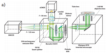
Figure 1a: Schematic diagram of the spinning disk confocal microscope modified for dual camera imaging with equal image sizes projected onto both sCMOS and EMCCD camera sensors (fluorescence emission pathway depicted only).
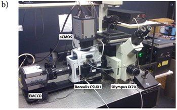
Figure 1b): Digital photograph of the modified confocal microscope.
Materials and Methods
Figure 1a depicts a schematic of the microscope apparatus we used for these studies. Fluorescence excited by a 491 nm laser and emitted by a microscopic sample was collected by a 60x, 1.40 NA oil immersion objective lens and imaged onto the pinhole disk of a modified Yokogawa CSU (model X1). This confocal image light was in turn re-collimated and relayed through the CSU scan head to a 50/50 beamsplitter which passes one half of the image light to the top camera port and the second half of the image light to the side camera port. (A subsequent control experiment showed that white light generated by the trans-illumination lamp of the inverted microscope was transmitted through the beamsplitter towards the sCMOS camera with an intensity that was only 2% greater than the light reflected from the beamsplitter towards the EMCCD camera.) The laser light was separated from the sample fluorescence in each light path by two identical Yokogawa green long-pass emission filters. A confocal fluorescence image of the sample was formed simultaneously on both cameras with two different adjustable camera lenses (EMCCD: 125 mm focal length; sCMOS: 50mm focal length). A shorter camera lens focal length was chosen for the sCMOS camera to demagnify the fluorescence image onto a sub-region the camera sensor and ensure that each pixel was exposed to an equal number of photons originating from the same area of the image that each pixel on the EMCCD was exposed to. The resultant image (de)magnification on each camera sensor could be finely adjusted with both camera lenses. The effective pixel dimensions backprojected onto the microscope sample plane were measured to be nearly identical (EMCCD: 235x235 nm2; sCMOS: 233x233 nm2). Figure 2 illustrates the process of extracting a 512x512 region of interest from the sCMOS camera image that matches the area imaged onto the full EMCCD camera chip. This experimental setup permitted a direct comparison of the camera sensitivities without the need for any pixel binning. Both cameras were computer operated using the freely available and open-source microscope control software MicroManager (version 1.4.8) [12, 13]. Typical EMCCD (Andor iXon3 DU-897) and sCMOS (Andor Neo) camera acquisition settings are shown in Figures 3 and 4 respectively.
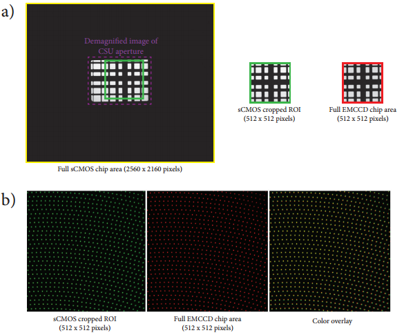
Figure 2: Registration and alignment of digital camera images. a) Image of an alignment grid slide projected onto the sCMOS camera using the 50 mm camera lens mounted on the top port of the CSUX1. Note that the entire CSU aperture can be viewed at this magnification (dashed purple outline). A 512x512 pixel region of interest is cropped from this image that matches the same area projected onto the EMCCD camera with the 125 mm camera lens mounted on the side port of the CSUX1. Both lenses are adjusted to yield equal pixel dimensions in the sample plane (as measured using MicroManager’s pixel calibrator plugin – sCMOS: 233x233 nm per pixel; EMCCD: 235x235 nm per pixel). b) The Borealis upgrade for the CSUX1 permits the axial position of both cameras to be translated to ensure that the cameras are perfectly focused onto the CSUX1 pinhole disk.

Figure 3 (left): EMCCD camera settings. Figure 4 (right): sCMOS camera settings
The sCMOS camera was operated in the rolling shutter mode. Image pixel intensities were converted from arbitrary digital units (ADUs) to photoelectron counts using the camera control software. All collected images were analyzed using the freely available open-source image processing software ImageJ (version 1.46f13) [14-16]. A full list of components and samples that comprised the apparatus and testing materials can be found in the Equipment List below.
Equipment List
Results:
Figure 5: Direct camera sensitivity comparison. a) An exposure image series of 1 μm diameter TetraSpeck fluorescent microspheres captured with the sCMOS and EMCCD digital cameras through the CSUX1. Each image in the series has been adjusted auto-contrasted. Below each image appears a horizontal line profile drawn through the central one microsphere in the image. Image dimensions: 50x50 pixels, scale bar = 1 μm. b) An exposure image series of two rat thoracic aorta myoblast cells captured with the sCMOS and EMCCD digital cameras through the CSUX1. FActin filaments inside the cells were fluorescently labeled with Bodipy-FL-phallacidin. Each image in the series has been adjusted auto contrasted. Below each image appears a histogram depicting the photoelectron distribution in the image. Image dimensions: 512x512 pixels, scale bar = 10 μm.
Figure 5a shows a series of images of 1 mm diameter fluorescent microspheres captured onto both cameras with increasing exposure time while holding the excitation laser power constant. These images and the accompanying line profiles clearly demonstrate that the EMCCD camera can detect the presence or absence of these small fluorescent objects at lower light levels compared to the sCMOS camera. As expected, at a certain light level, the images acquired by both cameras become visibly indistinguishable in quality. Figure 5b shows a similar image series of rat thoracic aorta myoblast cells where the F-actin filaments have been fluorescently labeled with Bodipy-FL (a green emitting fluorescent probe). Again, the photoelectron signal associated with these fluorescent objects clearly climbs above the background noise level on the EMCCD camera well before it does on the sCMOS camera. Assuming the camera manufacturer in this case has properly calibrated the ADU/photoelectron conversion factors on the detectors [17], the photoelectron image histograms of these images and the line profiles of the previous set of images suggest that the cross-over point in SNR performance occurs somewhere between 40 and 100 photoelectrons.
Discussion
Since their launch in 2010, there has been much speculation about whether sCMOS cameras will become a replacement for EMCCD cameras, which are currently considered the gold standard for low-light fluorescence microscopy and other bioimaging techniques. Our experiments have shown that even in the case of direct camera comparison with nearly equal light intensities presented to both cameras (<2% difference, no pixel binning), when compared to sCMOS cameras, EMCCD cameras are still able to produce superior, quantifiable images of fluorescent samples with pixel intensities of 40 photoelectrons or less.
It is important to remember, however, that throughout these experiments we have used highly stable test samples where the emitted fluorescence intensity can be arbitrarily changed over a few orders of magnitude simply by adjusting the laser power or camera exposure time. The cellular sample test slides contain fixed specimens with near perfect labeling of the structures of interest and with little to no background intensity. These properties of the test samples likely do not reflect the actual situation that is typically encountered in 3D spinning disk live-cell imaging experiments. In realistic situations like these, the fluorescent signal intensities are likely to be very weak. But just how many photons can one expect to be generated by a real, living cellular sample during a confocal imaging experiment? James Pawley has addressed this issue in the 2006 edition of his Hanbook of Biological Confocal Microscopy [18]. To quote directly: “Many users may find it hard to accept that the brightest pixel in their confocal images represents a signal of only 0–20 photons. The reason that a signal representing at most 8 photons is not displayed as a posterized image containing only 8 possible gray levels is that multiplicative noise in the image detector blends these 8 levels into each other so that the transitions are not apparent. Quite simply, some photoelectrons are counted as “more equal than others.” In fact, considerable experience shows that much fluorescence confocal microscopy is performed at much lower signal levels due to the low photon collection efficiency of most microscope systems. Indeed, the purpose of confocal imaging is to reject sample photons generated above and below the plane of focus to allow 3D optical sectioning! The geometric constraints also imposed by the numerical aperture of the objective lens as well as the inevitable losses in the optical train of the microscope lead to a loss of 80% or more of the original fluorescence signal. Depending on the properties of the detector, the resultant electronic signal may represent as little as 3% or as much as 16% of the total fluorescence emission.”
We must also be cognizant of the fact that fluorescent probe molecules can be destroyed by light (photobleaching), thereby creating phototoxic chemical products that kill the living cells under study. Live-cell spinning disk confocal imaging demands that we use low excitation light levels to produce useful fluorescence images and to keep the cells alive on the microscope stage at the same time. This important point has not been emphasized in any of the recent literature on sCMOS camera technology. A rule of thumb for minimization of photodynamic damage during live-cell imaging by reducing the excitation light intensity can be summarized as follows: “If you can see the fluorescence through the eyepieces, the excitation light is probably too bright” [19]. This again implies that the light levels presented to camera detectors in confocal microscopy should be very weak, somewhere in the 0-20 photons per pixel range. In reality, however, it is likely that many users of confocal microscopy actually do not abide by this rule of thumb and probably over-expose their living cellular samples to excitation light levels that produce more than 20 fluorescence photons per pixel, perhaps even at photon flux levels higher than the cross-over SNR point between sCMOS and EMCCD cameras. In addition, it is known that many spinning disk confocal microscope users choose to also use their instrument for fixed (ie: non-living) cellular specimen fluorescence imaging in which the need to reduce or minimize photodynamic damage can be neglected. In these cases it is very likely that the fixed specimen light levels reside near or above the cross-over point and an sCMOS camera for image detection would be more suitable than an EMCCD camera.
We return then to the original question that the R&D team of Spectral Applied Research set out to answer: Should one use an sCMOS or an EMCCD camera for spinning disk confocal microscopy? Since knowledge about a user’s typical sample light levels are key to choosing a camera type, this presents a bit of a chicken and egg problem: camera selection is dependent on this parameter but one needs a camera to measure it. Knowing the true SNR cross-over point between sCMOS and EMCCD cameras would aid in this decision since the user’s typical sample light levels could then be gauged against it.
Finally, recall that spatial resolution, temporal resolution, and feature signal intensity levels are all inter-related properties of an imaging system [20]. Bearing this fact in mind, let us consider the other purported benefits of sCMOS technology for spinning disk confocal microscopy. First, better intensity quantification capabilities can only be exploited when there is sufficient image signal to fill the entire dynamic range. As discussed above, this level of signal intensity is likely not present in live-cell imaging situations (when illuminated properly) and would require long exposure times. Second, high temporal resolution can only be achieved when the sample can again provide enough signal to allow images to be formed with sufficient detail at high frame rates. For the same reasons just given, the fast acquisition rates of sCMOS cameras cannot easily be exploited. In addition, it should be noted that even if the sample under study did provide sufficient signal for these high frame rates, the user would have to ensure that their spinning disk confocal system could rapidly rotate the pinhole disk to avoid the “scan line” artifact [21]. That is to say, the disk must rotate an integer number of disk sectors during the exposure time to avoid this artifact. Upgrades to the CSU system that allow the pinhole disk to spin at 5000 rpm or 10000 rpm can be purchased from Spectral Applied Research or Yokogawa, but even then the maximum possible frame rate that can be achieved without observing scan lines in the images is 1000 frames per second and 2000 frames per second respectively. Data demonstrating this fact and other notable rolling shutter-spinning disk effects were collected but not presented here. Lastly, it has been said that one of the benefits of sCMOS cameras over their EMCCD counterparts is their potential to achieve a better spatial resolution because of their smaller pixel size (which allows for proper Nyquist sampling of the confocal image). Proper Nyquist sampling of a confocal image captured with a 1.4 NA objective lens requires a sample plane pixel size of ~50x50 nm2 (see the Scientific Volume Imaging Nyquist calculator in reference [22]). In a retrospective study, we constructed a 215 mm sCMOS camera lens that magnifies the entire CSU image aperture over the full sCMOS sensor chip and achieves sample plane pixel dimensions of this size. The consequences of using such a camera lens on the CSU equipped with an sCMOS camera are illustrated in Figure 6. An improvement in lateral spatial resolution is possible with this lens (Figure 6d), but at the cost a ~17x increase in exposure time or excitation laser power! Living cells are not likely to tolerate such gains in excitation light or exposure, and so this mode of operation between the CSU and sCMOS camera is not recommended. To compensate, one might consider binning the expanded image, but this would reduce the spatial resolution and produce an image of inferior quality compared to that generated by the EMCCD with a normal CSU camera lens because of the increase in read noise associated with the binning operation on an sCMOS camera [4].
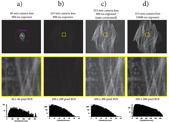
Figure 6: Consequences of expanding the CSU image aperture onto the full sCMOS chip area. a) Image of a fluorescently labeled rat thoracic aorta myoblast cell captured with the 50 mm camera lens onto the sCMOS camera through the CSU with a 900 ms exposure time. A dashed purple line outlines the CSU image aperture. Below the image appears a 46x46 pixel region of interest indicated by the yellow square drawn in the full image and its corresponding image histogram. b) The same cell is imaged onto the sCMOS camera through the CSU with the same exposure time and using a 215 mm camera lens that expands the image of the CSU aperture onto the full sCMOS camera chip (4.3x magnification). The contrast settings of this image are adjusted to be the same as in the image that appears in a). Below the full image appears a 200x200 pixel region of interest corresponding to the same region of interest area as in a), as well as the corresponding image histogram. c) The same images that appeared in b) auto-contrasted. d) A second image of the myoblast cell is captured using the 215 mm camera lens and with the exposure increased to 15000 ms. The contrast settings of this image are adjusted to be the same as in the image that appears in a). Note that the image histogram associated with the 200x200 pixel region of interest now shows a comparable photoelectron count distribution to the image histogram in a). While the image in d) possesses superior spatial resolution than the image in a), this has come at the cost of a ~17x increase in exposure time (alternatively the laser power could have been increased by the same factor using a 900 ms exposure time, possibly leading to accelerated photobleaching and cell death if the cell were alive, or fluorophore saturation effects which also lead to lower signal levels and increased photobleaching). This figure demonstrates the fundamental property that image brightness scales with the square of the image magnification onto the camera sensor.
Conclusion
Since it is impossible to know a priori the brightness exhibited by a user’s samples under typical imaging conditions and how this brightness level will compare to the cross-over SNR point between sCMOS and EMCCD camera technologies, we therefore still recommend the EMCCD camera as the camera of choice for spinning disk confocal microscopy. The ability to detect low signal intensities with low levels of illumination light power and form informative time-lapse images of dynamic cellular activities with EMCCD cameras outweighs the other benefits offered by sCMOS cameras at this point in time. An empirical measurement of the actual SNR cross-over point for these two camera technologies remains to be determined by us. Re-examination of sCMOS cameras for spinning disk confocal microscopy using a similar set of testing procedures will be necessary when their sensitivity can be enhanced by additional manufacturing processes (back-thinning of the sensor chip and better electronic read noise control for example).
References
Baker, M., Faster frames, clearer pictures. Nature Methods, 2011. 8(12): p. 1005-1009.
Joubert, J.R. and D.K. Sharma, EMCCD vs. sCMOS for Microscopic Imaging. Photonics Spectra, 2011. 45(3): p. 46-50.
Coates, C., EMCCD vs. sCMOS. Photonics Spectra, 2011. 45(5): p. 14-14.
Coates, C., NewsCMOSvs. Current Microscopy Cameras. Biophotonics International, 2011(May): p. 24-27.
Joubert, J.R., Y. Sabharwal, and D.K. Sharma, Digital Camera Technologies for Scientific Bio-Imaging. Part 3: Noise and Signal-to-Noise Ratios. Microscopy and Analysis, 2011(September).
Fullerton, S., et al. ORCA-Flash4.0: Changing the Game. 2011; Available from: http://hamamatsucameras.com/index.php
Sabharwal, Y., Digital Camera Technologies for Scientific Bio-Imaging. Part 4: SignaltoNoise Ratio and Image Comparison of Cameras. Microscopy and Analysis, 2012(January).
Tanaami, T., et al., High-speed 1-frame/ms scanning confocal microscope with a microlens and Nipkow disks. Applied Optics, 2002. 41(22): p. 4704-4708.
Inoue, S. and T. Inoue, Direct-view high-speed confocal scanner: The CSU-10, in Cell Biological Applications of Confocal Microscopy, Second Edition. 2002, Academic Press Inc: San Diego. p. 87-127.
Graf, R., J. Rietdorf, and T. Zimmermann, Live cell spinning disk microscopy, in Microscopy Techniques. 2005, Springer-Verlag Berlin: Berlin. p. 57-75.
Stuurman, N., N. Amodaj, and R.D. Vale, Micro-Manager: Open Source software for light microscope imaging. Microscopy Today, 2007. 15(3): p. 42-43.
Edelstein, A., et al., Computer Control of Microscopes Using μManager. 2010.
Abramoff, M.D., P.J. Magelhaes, and S.J. Ram, Image Processing with ImageJ. Biophotonics International, 2004. 11(7): p. 36-42.
Sheffield, J.B., ImageJ, a useful tool for biological image processing and analysis. Microscopy and Microanalysis, 2007. 13: p. 200-201.
Collins, T.J., ImageJ for microscopy. Biotechniques, 2007. 43(1): p. 25-30.
Janesick, J., CCD transfer method - Standard for absolute performance of CCDs and digital CCD camera systems. Solid State Sensor Arrays: Development and Applications, ed. M.M. Blouke. Vol. 3019. 1997, Bellingham: Spie - Int Soc Optical Engineering. 70-102.
Pawley, J., Handbook of Biological Confocal Microscopy. 3rd ed. 2006, New York: Plenum Press.
Spring, K.R., Cameras for digital microscopy, in Digital Microscopy, 3rd Edition, G. Sluder and D.E. Wolf, Editors. 2007, Elsevier Academic Press Inc: San Diego. p. 171-+
Dixon, A., T. Heinlein, and R. Wolleschensky, Need for Standardization of Fluorescence Measurements from the Instrument Manufacturer’s View Standardization and Quality Assurance in Fluorescence Measurements II. 2008. 6: p. 3-24.
Chong, F.K., et al., Optimization of spinning disk confocal microscopy: Synchronization with the ultra-sensitive EMCCD, in Three-Dimensional and Multidimensional Microscopy: Image Acquisition and Processing Xi, J.A. Conchello, C.H. Cogswell, and T. Wilson, Editors. 2004, Spie-Int Soc Optical Engineering: Bellingham. p. 65-76.
SVI Nyquist Calculator. Available from: http://www.svi.nl/NyquistCalculator.
© Oxford Instruments 2024